40 multiple data labels excel pie chart
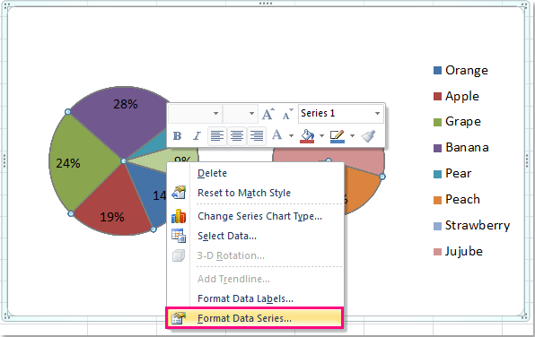
How to Create and Format a Pie Chart in Excel - Lifewire Select the plot area of the pie chart. Right-click the chart. Select Add Data Labels . Select Add Data Labels. In this example, the sales for each cookie is added to the slices of the pie chart. Change Colors, When a chart is created in Excel, or whenever an existing chart is selected, two additional tabs are added to the ribbon. Pie Chart in Excel - Inserting, Formatting, Filters, Data Labels Click on the Instagram slice of the pie chart to select the instagram. Go to format tab. (optional step) In the Current Selection group, choose data series "hours". This will select all the slices of pie chart. Click on Format Selection Button. As a result, the Format Data Point pane opens.
Pie Chart Examples | Types of Pie Charts in Excel with Examples PIE Chart can be defined as a circular chart with multiple divisions in it, ... Right-click and choose the “Add Data Labels “option for additional drop-down options. ... Here we discuss Types of Pie Chart in Excel along with practical examples and downloadable excel template.
Multiple data labels excel pie chart
Quickly create multiple progress pie charts in one graph - ExtendOffice 1. Click Kutools > Charts > Difference Comparison > Progress Pie Chart to go to the Progress Pie Chart dialog box. 2. In the popped out dialog box, select the data range of the axis labels, actual values and target values under the Axis Labels, Actual Value and Target Value boxes separately. See screenshot: How to Combine or Group Pie Charts in Microsoft Excel Click on the first chart and then hold the Ctrl key as you click on each of the other charts to select them all. Click Format > Group > Group. All pie charts are now combined as one figure. They will move and resize as one image. Choose Different Charts to View your Data, How to create a chart in Excel from multiple sheets Nov 05, 2015 · If you want to plot data from multiple worksheets in your graph, repeat the process described in step 2 for each data series you want to add. When done, click the OK button on the Select Data Source dialog window. In this example, I've added the 3 rd data series, here's how my Excel chart looks now: 4. Customize and improve the chart (optional)
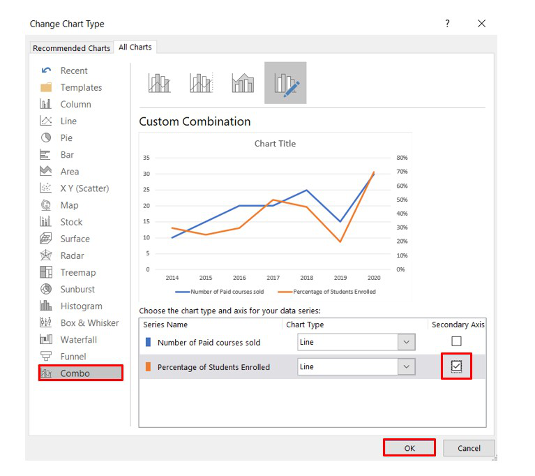
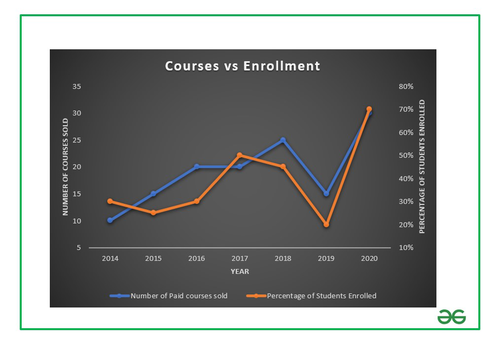
Multiple data labels excel pie chart. Pie Chart Examples | Types of Pie Charts in Excel with Examples PIE Chart can be defined as a circular chart with multiple divisions in it, and each division represents some portion of a total circle or total value. Simply each circle represents the total value of 100 per cent, and each division contributes some per cent to the total. Multiple Data Labels on a Pie Chart | MrExcel Message Board Hello All, So I have a table with 8 rows and 3 columns. This table includes: Column 1 - shipment name. Column 2 - shipment cost. Column 3 - shipment weight. I have created a pie chart from this table, which covers the first two columns. Displayed next to each slice is a label with the shipment name, shipment cost, and percent share of the pie. Plot Multiple Data Sets on the Same Chart in Excel 29-06-2021 · Select the Chart -> Design -> Change Chart Type. Another way is : Select the Chart -> Right Click on it -> Change Chart Type. 2. The Chart Type dialog box opens. Now go to the “Combo” option and check the “Secondary Axis” box for the “Percentage of Students Enrolled” column.This will add the secondary axis in the original chart and will separate the two charts. How to create a chart in Excel from multiple sheets - Ablebits.com 05-11-2015 · If you want to plot data from multiple worksheets in your graph, repeat the process described in step 2 for each data series you want to add. When done, click the OK button on the Select Data Source dialog window. In this example, I've added the 3 rd data series, here's how my Excel chart looks now: 4. Customize and improve the chart (optional)
Create a multi-level category chart in Excel - ExtendOffice Select the dots, click the Chart Elements button, and then check the Data Labels box. 23. Right click the data labels and select Format Data Labels from the right-clicking menu. 24. In the Format Data Labels pane, please do as follows. 24.1) Check the Value From Cells box; Select data for a chart - support.microsoft.com Pie chart. This chart uses one set of values (called a data series). Learn more about. pie charts. In one column or row, and one column or row of labels. Doughnut chart. This chart can use one or more data series. Learn more about. doughnut charts. In one or multiple columns or rows of data, and one column or row of labels. XY (scatter) or ... How To Make A Pie Chart In Excel. - Spreadsheeto How To Make A Pie Chart In Excel. In Just 2 Minutes! Written by co-founder Kasper Langmann, Microsoft Office Specialist. The pie chart is one of the most commonly used charts in Excel. Why? Because it’s so useful 🙂. Pie charts can show a lot of information in a small amount of space. They primarily show how different values add up to a whole. How to Make a Pie Chart in Excel & Add Rich Data Labels to ... Sep 08, 2022 · In this article, we are going to see a detailed description of how to make a pie chart in excel. One can easily create a pie chart and add rich data labels, to one’s pie chart in Excel. So, let’s see how to effectively use a pie chart and add rich data labels to your chart, in order to present data, using a simple tennis related example.
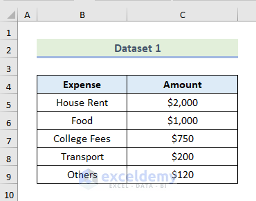
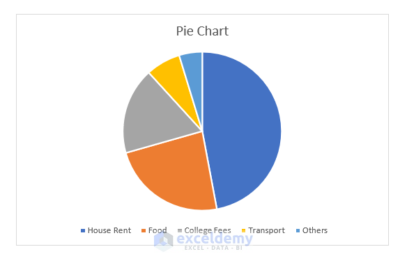
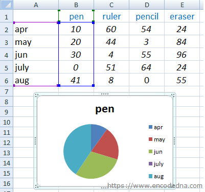
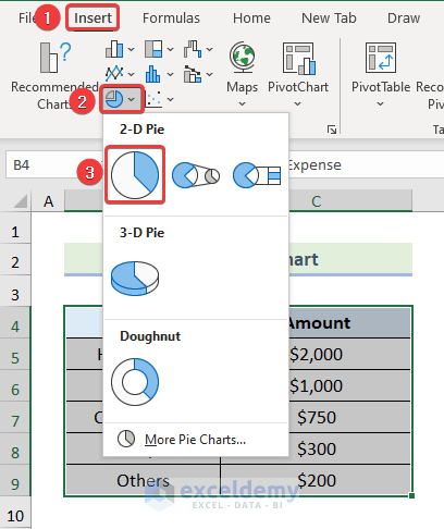
Show multiple data lables on a chart - Power BI For example, I'd like to include both the total and the percent on pie chart. Or instead of having a separate legend include the series name along with the % in a pie chart. I know they can be viewed as tool tips, but this is not sufficient for my needs. Many of my charts are copied to presentations and this added data is necessary for the end ... Comparison Chart in Excel | Adding Multiple Series ... - EDUCBA This window helps you modify the chart as it allows you to add the series (Y-Values) as well as Category labels (X-Axis) to configure the chart as per your need. Under Legend Entries ( S eries) inside the Select Data Source window, you need to select the sales values for the year 2018 and year 2019. How to Show Percentage in Pie Chart in Excel? - GeeksforGeeks 29-06-2021 · Select a 2-D pie chart from the drop-down. A pie chart will be built. Select -> Insert -> Doughnut or Pie Chart -> 2-D Pie. Initially, the pie chart will not have any data labels in it. To add data labels, select the chart and then click on the “+” button in the top right corner of the pie chart and check the Data Labels button. How to Make a Pie Chart with Multiple Data in Excel (2 Ways) - ExcelDemy Steps: First, select the dataset and go to the Insert tab from the ribbon. After that, click on Insert Pie or Doughnut Chart from the Charts group. Afterward, from the drop-down choose the 1st Pie Chart among the 2-D Pie.
Move and Align Chart Titles, Labels, Legends with the Arrow ...
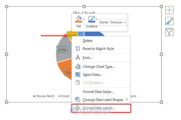
Excel Pie Chart Labels on Slices: Add, Show & Modify Factors - ExcelDemy It will help us to separate the data labels from the pie chart. 📌 Steps: First of all, click on the data labels on the pie chart. Now, in the Format tab, click on the drop-down arrow of the Shape Outline from the Shapes Style group. Then, choose your desired color for the shape outline. We choose White, Background 1 color for our shape outline.
EXCEL Charts: Column, Bar, Pie and Line
How to Show Percentage and Value in Excel Pie Chart - ExcelDemy From the Chart Element option, click on the Data Labels. These are the given results showing the data value in a pie chart. Right-click on the pie chart. Select the Format Data Labels command. Now click on the Value and Percentage options. Then click on the anyone of Label Positions. Here, we will click the Best Fit option.

Creating Graphs in Excel 2013
Adding second set of data labels - Excel Help Forum Re: Adding second set of data labels. The chart links to workbooks on your hard drive, not to the data in the sheet. The secondary axis can only be shown when there is a series plotting on the secondary axis. Both your series are plotted on the first axis. You need to select the COUNT OF PARTS series, format it and send it to the secondary axis.

Power BI Pie Chart - Complete Tutorial - EnjoySharePoint
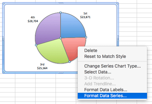
Creating Pie Chart and Adding/Formatting Data Labels (Excel) Creating Pie Chart and Adding/Formatting Data Labels (Excel) Creating Pie Chart and Adding/Formatting Data Labels (Excel)

Excel charts: add title, customize chart axis, legend and ...
How to Make a Pie Chart in Excel & Add Rich Data Labels to The Chart! 08-09-2022 · A pie chart is used to showcase parts of a whole or the proportions of a whole. There should be about five pieces in a pie chart if there are too many slices, then it’s best to use another type of chart or a pie of pie chart in order to showcase the data better. In this article, we are going to see a detailed description of how to make a pie chart in excel.

How to Make a Pie Chart in Excel – Contextures Blog
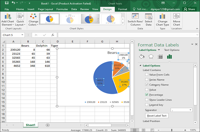
Change the format of data labels in a chart To format data labels, select your chart, and then in the Chart Design tab, click Add Chart Element > Data Labels > More Data Label Options. Click Label Options and under Label Contains , pick the options you want.
How to create pie of pie or bar of pie chart in Excel?
Multiple data labels (in separate locations on chart) Re: Multiple data labels (in separate locations on chart) You can do it in a single chart. Create the chart so it has 2 columns of data. At first only the 1 column of data will be displayed. Move that series to the secondary axis. You can now apply different data labels to each series. Attached Files, 819208.xlsx (13.8 KB, 265 views) Download,
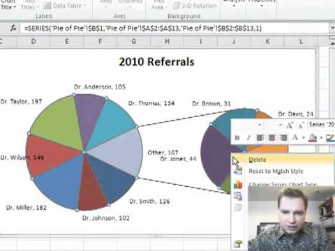
Excel Video 128 Pie of Pie Charts
How to add two data labels for the same data on a pie chart? : excel On the "Dashboard" sheet create a white circle and lay it over your circle graph. Right click it and select "Edit Text." When the cursor appears, click the formula bar and enter: =Calculation!C1. Format and align the text as desired. Next make a text box beneath the pie chart and using the same method as above set the text equal to Calculation ...
How to make a pie chart in Excel
How To Make A Pie Chart In Excel: In Just 2 Minutes [2022] When you first create a pie chart, Excel will use the default colors and design.. But if you want to customize your chart to your own liking, you have plenty of options. The easiest way to get an entirely new look is with chart styles.. In the Design portion of the Ribbon, you’ll see a number of different styles displayed in a row. Mouse over them to see a preview:

How to Create a Pie Chart in Excel | Smartsheet
How to show percentage in pie chart in Excel? - ExtendOffice Show percentage in pie chart in Excel. Please do as follows to create a pie chart and show percentage in the pie slices. 1. Select the data you will create a pie chart based on, click Insert > Insert Pie or Doughnut Chart > Pie. See screenshot: 2. Then a pie chart is created. Right click the pie chart and select Add Data Labels from the context ...
How to Make a Pie Chart with Multiple Data in Excel (2 Ways)
How to display leader lines in pie chart in Excel? - ExtendOffice To display leader lines in pie chart, you just need to check an option then drag the labels out. 1. Click at the chart, and right click to select Format Data Labels from context menu. 2. In the popping Format Data Labels dialog/pane, check Show Leader Lines in the Label Options section. See screenshot: 3. Close the dialog, now you can see some ...

Automatically Group Smaller Slices in Pie Charts to one big Slice
Pie Charts in Excel - How to Make with Step by Step Examples Step 3: Right-click the pie chart and expand the "add data labels" option. Next, choose "add data labels" again, as shown in the following image. Step 4: The data labels are added to the chart, as shown in the following image. With these labels, the sales quantity of each flavor is displayed on the respective slice.

How to Show Percentage in Pie Chart in Excel? - GeeksforGeeks
How to add data labels from different column in an Excel chart? This method will guide you to manually add a data label from a cell of different column at a time in an Excel chart. 1. Right click the data series in the chart, and select Add Data Labels > Add Data Labels from the context menu to add data labels. 2. Click any data label to select all data labels, and then click the specified data label to select it only in the chart.
Plot Multiple Data Sets on the Same Chart in Excel ...
Move data labels - support.microsoft.com Right-click the selection > Chart Elements > Data Labels arrow, and select the placement option you want. Different options are available for different chart types. For example, you can place data labels outside of the data points in a pie chart but not in a column chart.

Improve your X Y Scatter Chart with custom data labels
How to display leader lines in pie chart in Excel? - ExtendOffice To display leader lines in pie chart, you just need to check an option then drag the labels out. 1. Click at the chart, and right click to select Format Data Labels from context menu. 2. In the popping Format Data Labels dialog/pane, check Show Leader Lines in the Label Options section. See screenshot: 3. Close the dialog, now you can see some ...
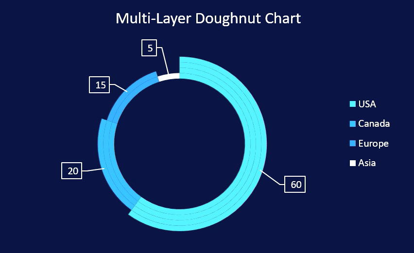
How to create a creative multi-layer Doughnut Chart in Excel
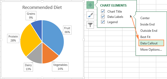
Add or remove data labels in a chart - support.microsoft.com Click the data series or chart. To label one data point, after clicking the series, click that data point. In the upper right corner, next to the chart, click Add Chart Element > Data Labels. To change the location, click the arrow, and choose an option. If you want to show your data label inside a text bubble shape, click Data Callout.
How to Make a Pie Chart in Excel 2010, 2013, 2016?
Plot Multiple Data Sets on the Same Chart in Excel ... Jun 29, 2021 · Select the Chart -> Design -> Change Chart Type. Another way is : Select the Chart -> Right Click on it -> Change Chart Type. 2. The Chart Type dialog box opens. Now go to the “Combo” option and check the “Secondary Axis” box for the “Percentage of Students Enrolled” column.
How to Make a Pie Chart with Multiple Data in Excel (2 Ways)
Edit titles or data labels in a chart - support.microsoft.com To edit the contents of a title, click the chart or axis title that you want to change. To edit the contents of a data label, click two times on the data label that you want to change. The first click selects the data labels for the whole data series, and the second click selects the individual data label. Click again to place the title or data ...
Automatically Group Smaller Slices in Pie Charts to one big Slice
How to add or move data labels in Excel chart? - ExtendOffice In Excel 2013 or 2016. 1. Click the chart to show the Chart Elements button . 2. Then click the Chart Elements, and check Data Labels, then you can click the arrow to choose an option about the data labels in the sub menu. See screenshot: In Excel 2010 or 2007. 1. click on the chart to show the Layout tab in the Chart Tools group. See ...
How to Make a Pie Chart with Multiple Data in Excel (2 Ways)
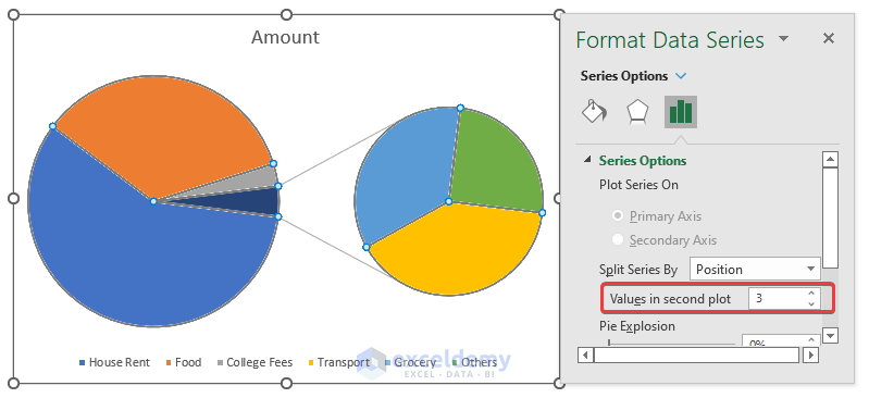
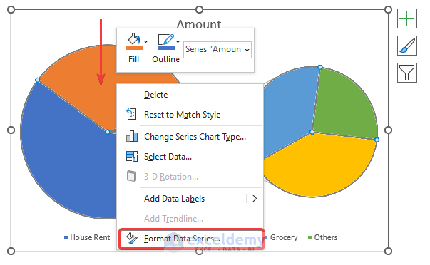
How to Make Pie of Pie Chart in Excel (with Easy Steps) Expand a Pie of Pie Chart in Excel. You can do an interesting thing with a Pie of Pie Chart in Excel. Which is explode of the Pie of Pie Chart in Excel. The steps to expand a Pie of Pie Chart are given below. Steps: Firstly, you must select the data range. Here, I have selected the range B4:C12. Secondly, you have to go to the Insert tab.
How to Make a Pie Chart with Multiple Data in Excel (2 Ways)
updating data labels in pie charts, - Microsoft Community The data labels in my pie chart won't update. My data labels use & to combine data from three cells into a label and the result is the data label. ... Excel / For business / Windows; What's new. Surface Laptop Go 2; Surface Pro 8; Surface Laptop Studio; Surface Pro X; Surface Go 3; Surface Duo 2; Surface Pro 7+

Add or remove data labels in a chart
Comparison Chart in Excel | Adding Multiple Series Under Same … This window helps you modify the chart as it allows you to add the series (Y-Values) as well as Category labels (X-Axis) to configure the chart as per your need. Under Legend Entries ( S eries) inside the Select Data Source window, you need to select the …

How to show data labels in PowerPoint and place them ...
How to create a chart in Excel from multiple sheets Nov 05, 2015 · If you want to plot data from multiple worksheets in your graph, repeat the process described in step 2 for each data series you want to add. When done, click the OK button on the Select Data Source dialog window. In this example, I've added the 3 rd data series, here's how my Excel chart looks now: 4. Customize and improve the chart (optional)
How to Create a Pie Chart in Excel using Worksheet Data
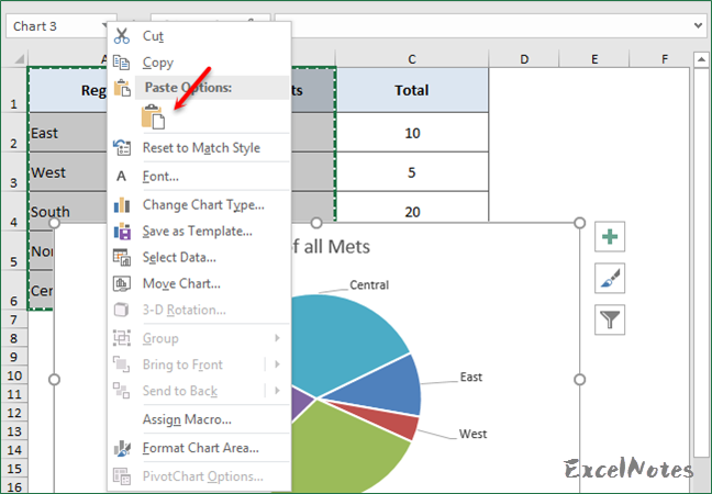
How to Combine or Group Pie Charts in Microsoft Excel Click on the first chart and then hold the Ctrl key as you click on each of the other charts to select them all. Click Format > Group > Group. All pie charts are now combined as one figure. They will move and resize as one image. Choose Different Charts to View your Data,
How to Make a Pie Chart with Multiple Data in Excel (2 Ways)
Quickly create multiple progress pie charts in one graph - ExtendOffice 1. Click Kutools > Charts > Difference Comparison > Progress Pie Chart to go to the Progress Pie Chart dialog box. 2. In the popped out dialog box, select the data range of the axis labels, actual values and target values under the Axis Labels, Actual Value and Target Value boxes separately. See screenshot:
Plot Multiple Data Sets on the Same Chart in Excel ...
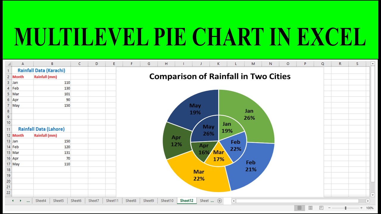
How to Make Multilevel Pie Chart in Excel
How to Create a Pie Chart in Excel | Smartsheet

Excel charts: add title, customize chart axis, legend and ...

How to Add Two Data Labels in Excel Chart (with Easy Steps ...
How to Make a Pie Chart with Multiple Data in Excel (2 Ways)

excel - Finding multiple local maxima and placing data labels ...

EXCEL Charts: Column, Bar, Pie and Line

Plot Multiple Data Sets on the Same Chart in Excel ...

Creating Pie Chart and Adding/Formatting Data Labels (Excel)
How to Make Pie Chart with Labels both Inside and Outside ...

How to create pie of pie or bar of pie chart in Excel?
Excel macro to fix overlapping data labels in line chart ...

Best Excel Tutorial - Multi Level Pie Chart

How to Make Pie Chart with Labels both Inside and Outside ...
Post a Comment for "40 multiple data labels excel pie chart"