44 excel chart custom data labels

How to: Display and Format Data Labels - DevExpress Apply Number Format to Data Labels Create a Custom Label Entry After you create a chart, you can add a data label to each data point in the chart to identify its actual value. By default, data labels are linked to data that the chart uses. When data changes, information in the data labels is updated automatically. How to Print Labels from Excel - Lifewire Choose Start Mail Merge > Labels . Choose the brand in the Label Vendors box and then choose the product number, which is listed on the label package. You can also select New Label if you want to enter custom label dimensions. Click OK when you are ready to proceed. Connect the Worksheet to the Labels

How to Create and Customize a Waterfall Chart in Microsoft Excel Select the chart and use the buttons on the right (Excel on Windows) to adjust Chart Elements like labels and the legend, or Chart Styles to pick a theme or color scheme. Select the chart and go to the Chart Design tab. Then, use the tools in the ribbon to select a different layout, change the colors, pick a new style, or adjust your data ...

Excel chart custom data labels

chandoo.org › wp › change-data-labels-in-chartsHow to Change Excel Chart Data Labels to Custom Values? May 05, 2010 · First add data labels to the chart (Layout Ribbon > Data Labels) Define the new data label values in a bunch of cells, like this: Now, click on any data label. This will select “all” data labels. Now click once again. At this point excel will select... Go to Formula bar, press = and point to the ... Pie Chart in Excel - Inserting, Formatting, Filters, Data Labels Click on the Instagram slice of the pie chart to select the instagram. Go to format tab. (optional step) In the Current Selection group, choose data series "hours". This will select all the slices of pie chart. Click on Format Selection Button. As a result, the Format Data Point pane opens. Format Chart Axis in Excel - Axis Options Right-click on the Vertical Axis of this chart and select the "Format Axis" option from the shortcut menu. This will open up the format axis pane at the right of your excel interface. Thereafter, Axis options and Text options are the two sub panes of the format axis pane. Formatting Chart Axis in Excel - Axis Options : Sub Panes

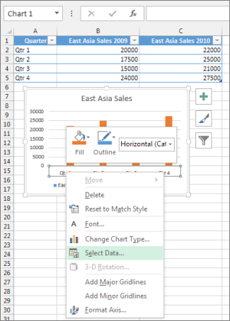
Excel chart custom data labels. DataLabels.Separator property (Excel) | Microsoft Docs This example sets the data label separator for the first series on the first chart to a semicolon. This example assumes that a chart exists on the active worksheet. VB Copy Sub ChangeSeparator () ActiveSheet.ChartObjects (1).Chart.SeriesCollection (1) _ .DataLabels.Separator = ";" End Sub Support and feedback support.microsoft.com › en-us › officeEdit titles or data labels in a chart - support.microsoft.com The first click selects the data labels for the whole data series, and the second click selects the individual data label. Right-click the data label, and then click Format Data Label or Format Data Labels. Click Label Options if it's not selected, and then select the Reset Label Text check box. Top of Page › custCustom data labels in a chart - Get Digital Help Jan 21, 2020 · Press with right mouse button on on any data series displayed in the chart. Press with mouse on "Add Data Labels". Press with mouse on Add Data Labels". Double press with left mouse button on any data label to expand the "Format Data Series" pane. Enable checkbox "Value from cells". Custom data labels pop-ups after hovering mouse over a scatter chart Currently with Excel charts I can have either (a) some information after mouse hovering or (b) custom data in my label but displayed constantly. a) hover label.png b) custom lavel.PNG The problem with both is that it'll be way too many data for a typical label, and the 'temporary label' seen after mouse hovering won't give me the data I need.

5 New Charts to Visually Display Data in Excel 2019 - dummies Enter the labels and data. Put them in the order you want them to appear in the chart, from top to bottom. You can convert the range to a table to sort it more easily. Select the labels and data and then click Insert → Insert Waterfall, Funnel, Stock, Surface, or Radar Chart → Funnel. Format the chart as desired. How to Create and Customize a Pareto Chart in Microsoft Excel Go to the Insert tab and click the "Insert Statistical Chart" drop-down arrow. Select "Pareto" in the Histogram section of the menu. Remember, a Pareto chart is a sorted histogram chart. And just like that, a Pareto chart pops into your spreadsheet. You'll see your categories as the horizontal axis and your numbers as the vertical axis. Excel Waterfall Chart: How to Create One That Doesn't Suck Click inside the data table, go to " Insert " tab and click " Insert Waterfall Chart " and then click on the chart. Voila: OK, technically this is a waterfall chart, but it's not exactly what we hoped for. In the legend we see Excel 2016 has 3 types of columns in a waterfall chart: Increase. Decrease. How to Make a Pie Chart in Excel & Add Rich Data Labels to The Chart! 7) With the data point still selected, go to Chart Tools>Format>Shape Styles and click on the drop-down arrow next to Shape Effects and select Shadow and choose Inner Shadow>Inside Diagonal Top Left. 8) With the one data point still selected, right-click this data point, and select Add Data Label>Add Data Callout as shown below.

How to Create and Customize a Treemap Chart in Microsoft Excel Either right-click the chart and pick "Format Chart Area" or double-click the chart to open the sidebar. On Windows, you'll see two handy buttons on the right of your chart when you select it. With these, you can add, remove, and reposition Chart Elements. And you can pick a style or color scheme with the Chart Styles button. Custom Chart Data Labels In Excel With Formulas Jan 07, 2022 · Follow the steps below to create the custom data labels. Select the chart label you want to change. In the formula-bar hit = (equals), select the cell reference containing your chart label’s data. In this case, the first label is in cell E2. Finally, repeat for all your chart laebls. Modifying Axis Scale Labels (Microsoft Excel) Follow these steps: Create your chart as you normally would. Double-click the axis you want to scale. You should see the Format Axis dialog box. (If double-clicking doesn't work, right-click the axis and choose Format Axis from the resulting Context menu.) Make sure the Number tab is displayed. (See Figure 1.) Figure 1. Line Chart corrupted when custom X-axis labels assigned. [MacOS, Excel 2016 update 2021-07-31] I have a line chart with a LOT of Y data values (1000+), and the chart looks fine until I try to set the X axis labels (they default to the sequence 1...#data points). When I do this, Excel changes my graph type to, what looks like, a bar chart with a single bar on it. Has anyone had this issue?

How to Make Charts and Graphs in Excel | Smartsheet

Custom Excel number format - Ablebits.com To create a custom Excel format, open the workbook in which you want to apply and store your format, and follow these steps: Select a cell for which you want to create custom formatting, and press Ctrl+1 to open the Format Cells dialog. Under Category, select Custom. Type the format code in the Type box. Click OK to save the newly created format.

Displaying Numbers in Thousands in a Chart in Microsoft Excel | Microsoft Excel Tips from Excel ...

How to Add Data Table in an Excel Chart (4 Quick Methods) 4 Methods for Data Table in Excel Chart 1. Add Data Table From Chart Design Tab in Excel 1.1. Show Data Table Using 'Quick Layout' Option 1.2. Use the 'Add Chart Element' Option to Show Data Tables 2. Show/Hide Data Table by Clicking the Plus (+) Sign of Excel Chart 3. Add Extra Data Series to Data Table but Not in Chart 4.

Change axis labels in a chart - Office Support

How to Apply a Filter to a Chart in Microsoft Excel Go to the Home tab, click the Sort & Filter drop-down arrow in the ribbon, and choose "Filter.". Click the arrow at the top of the column for the chart data you want to filter. Use the Filter section of the pop-up box to filter by color, condition, or value. When you finish, click "Apply Filter" or check the box for Auto Apply to see ...

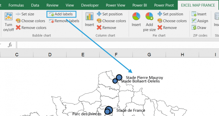
How to geocode customer addresses and show them on an Excel bubble chart? – Maps for Excel ...

DataLabels object (Excel) | Microsoft Docs Use the DataLabels method of the Series object to return the DataLabels collection. The following example sets the number format for data labels on series one on chart sheet one. VB Copy With Charts (1).SeriesCollection (1) .HasDataLabels = True .DataLabels.NumberFormat = "##.##" End With

Show Trend Arrows in Excel Chart Data Labels

Custom data label color based on another cell Value (Priority) You can do this, by using conditional formatting (just as you maybe have other places in the Gantt Chart). Mark the area you will use, and in conditional format choose, "New rule" and insert: IF (A$1=1;TRUE). A1 has to reflect the cell you have the value in, and 1 in the formula, are the value you will use. SereneSea New Member Joined Feb 2, 2022

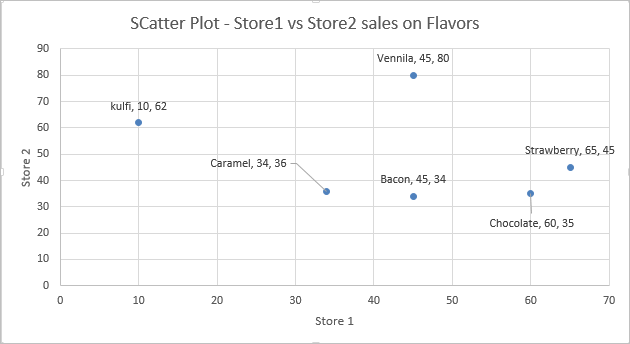
Add Custom Labels to x-y Scatter plot in Excel - DataScience Made Simple

support.microsoft.com › en-us › officeAdd or remove data labels in a chart - support.microsoft.com Add data labels to a chart Click the data series or chart. To label one data point, after clicking the series, click that data point. In the upper right corner, next to the chart, click Add Chart Element > Data Labels. To change the location, click the arrow, and choose an option. If you want to ...

microsoft excel - How to make chart showing year over year, where fiscal year starts July ...

6 Tips for Making Microsoft Excel Charts That Stand Out Select the Right Chart for the Data. The first step in creating a chart or graph is selecting the one that best fits your data. You can gain a lot of insight on this by looking at Excel's suggestions. Select the data you want to plot on a chart. Then, head to the Insert tab and Charts section of the ribbon.

Share :