45 excel pivot table column labels
Pivot Table column label from horizontal to vertical Pivot Table column label from horizontal to vertical After pivot table and with grouping, some column labels have been showed but the caption is on the top. What i want is put the column header at the left of the row as vertical red text show as below. However, i cannot do this, it said "We cant change this part of pivot table". Design the layout and format of a PivotTable In the PivotTable, right-click the row or column label or the item in a label, point to Move, and then use one of the commands on the Move menu to move the item to another location. Select the row or column label item that you want to move, and then point to the bottom border of the cell.
Excel 2016 Pivot table Row and Column Labels - Microsoft Community Mar 15, 2018 · In Excel 2016 I’ve found when I create a pivot table it unhelpfully shows ‘Row Labels’ and ‘Column Labels’ instead of my field names, although in the top left cell it says ‘Count of’ and then inserts the correct field name. Years ago when I last used Excel it automatically put the field names in all three heading cells.

Excel pivot table column labels
How to Format Excel Pivot Table - Contextures Excel Tips 23/05/2022 · Keep Formatting in Excel Pivot Table. A pivot table is automatically formatted with a default style when you create it, and you can select a different style later, or add your own formatting. For example, in the pivot table shown below, colour has been added to the subtotal rows, and column B is narrow. Formatting Disappears. However, some of that pivot table … How to insert a blank column in pivot table? - Chandoo.org 16/04/2015 · We all know pivot table functionality is a powerful & useful feature. But it comes with some quirks. For example, we cant insert a blank row or column inside pivot tables. So today let me share a few ideas on how you can insert a blank column. But first let's try inserting a column Imagine you are looking at a pivot table like above. And you want to insert a column or row. … Pivot table row labels side by side - Excel Tutorials You can copy the following table and paste it into your worksheet as Match Destination Formatting. Now, let's create a pivot table ( Insert >> Tables >> Pivot Table) and check all the values in Pivot Table Fields. Fields should look like this. Right-click inside a pivot table and choose PivotTable Options…. Check data as shown on the image below.
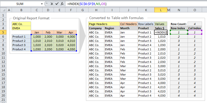
Excel pivot table column labels. Combining Column Values in an Excel Pivot Table - Stack Overflow 14/05/2018 · In order to simplify a stacked bar chart, I am looking to sum up the counts of multiple columns I have in my pivot table. For example, in this sample table, I would like to combine Fruits and Vegetables into one column, so that each bar will comprised of three colors: one for Meats, one for Grains, and one for Fruits+Vegetables. Hide Pivot Table Buttons and Labels - Contextures Blog Right-click a cell in the pivot table and, in the pop up menu, click PivotTable Options. In the Display section, remove the check mark from Show Expand/Collapse Buttons. This change will hide the Expand/Collapse buttons to the left of the outer Row Labels and Column Labels. Next, remove the check mark from Display Field Captions and Filter Drop ... Use column labels from an Excel table as the rows in a Pivot Table Highlight your current table, including the headers Then from the Data section of the ribbon, select From Table Highlight all the columns containing data, but not the Year column, and then select Unpivot Columns Close the dialog and keep the changes. Excel should place the unpivoted data into a new worksheet, looking something like this: Excel Pivot values as column labels - Stack Overflow If you have Excel for Office 365 (or Excel 2021) with the FILTER function, you can use the following: Note that I used a table with structured references for the data source. This has advantages in editing the table in the future. For "pivot" header: =TRANSPOSE(SORT(UNIQUE(Table1[Country]))) For the columns:
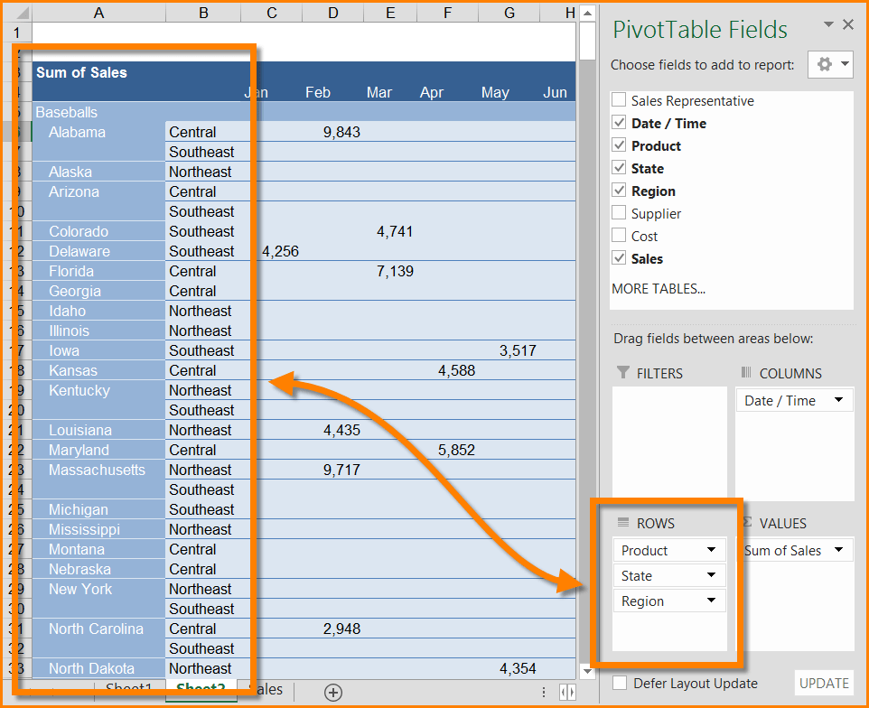
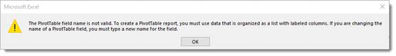
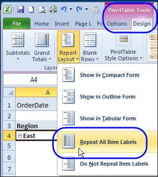
Excel Pivot Table Group: Step-By-Step Tutorial To Easily Group … Let's start by looking at the… Example Pivot Table And Source Data. This Pivot Tutorial is accompanied by an Excel workbook example. If you want to follow each step of the way and see the results of the processes I explain below, you can get immediate free access to this workbook by subscribing to the Power Spreadsheets Newsletter.. I use the following source data for all … Repeat All Item Labels In An Excel Pivot Table - MyExcelOnline DOWNLOAD EXCEL WORKBOOK. STEP 1: Click in the Pivot Table and choose PivotTable Tools > Options (Excel 2010) or Design (Excel 2013 & 2016) > Report Layouts > Show in Outline/Tabular Form STEP 2: Now to fill in the empty cells in the Row Labels you need to select PivotTable Tools > Options (Excel 2010) or Design (Excel 2013 & 2016) > Report Layouts > Repeat All Item Labels Expand Pivot Table Column labels vertically / downwards Expand Pivot Table Column labels vertically / downwards As we know we can expand/collapse Row Headers or Column Headers in Pivot Tables to reveal details. When we expand column headers, it expands rightwards. My objective is to make it expand downwards (vertically). Repeat item labels in a PivotTable - support.microsoft.com Right-click the row or column label you want to repeat, and click Field Settings. Click the Layout & Print tab, and check the Repeat item labels box. Make sure Show item labels in tabular form is selected. Notes: When you edit any of the repeated labels, the changes you make are applied to all other cells with the same label.
Excel tutorial: How to filter a pivot table by rows or columns When you add a field as a row or column label in a pivot table, you automatically get the ability to filter the results in the table by items that appear in that field. Let's take a look. This pivot table is displaying just one field: Total Sales. After we add Product as a row label, notice that a drop-down arrow appears in the header area. How to group time by hour in an Excel pivot table? Right-click any time in the Row Labels column, and select Group in the context menu. See screenshot: 5. In the Grouping dialog box, please click to highlight Hours only in the By list box, and click the OK button. See screenshot: Now the time data is grouped by hours in the newly created pivot table. See screenshot: Note: If you need to group time data by days and hours … How to Create Excel Pivot Table [Includes practice file] 15/01/2022 · Using an Excel pivot table, you can organize and group the same data in ways that start to answer actionable questions like: ... There are also ways to filter the data using the controls next to Row Labels or Column labels on the pivot table. You may also drag fields to the Report Filter quadrant. Troubleshooting Excel Pivot Tables . You might encounter several … How to Create a Pivot Table in Excel: A Step-by-Step Tutorial 31/12/2021 · Every pivot table in Excel starts with a basic Excel table, where all your data is housed. To create this table, simply enter your values into a specific set of rows and columns. Use the topmost row or the topmost column to categorize your values by what they represent. For example, to create an Excel table of blog post performance data, you might have a …
How to Sort Pivot Table Row Labels, Column Field Labels and Data Values with Excel VBA Macro ...
How to make row labels on same line in pivot table? Make row labels on same line with PivotTable Options You can also go to the PivotTable Options dialog box to set an option to finish this operation. 1. Click any one cell in the pivot table, and right click to choose PivotTable Options, see screenshot: 2.
Excel - Mixed Pivot Table Layout | SkillForge
Excel Pivot Table with multiple columns of data and each data … 17/04/2019 · To start, I replicated your dataset and set it up as a table: Then I made multiple Pivot Tables, filling the Columns and Values Pivot Table Fields with one Category of each of your categories. This will produce a Pivot Table with 3 rows. The first row will read Column Labels with a filter dropdown. The second row will read all the possible ...

Quick Pivot Tables in Excel with QuickBooks Data - Export Excel to QuickBooks - Experts in ...
Pivot table - Wikipedia Column labels are used to apply a filter to one or more columns that have to be shown in the pivot table. For instance if the "Salesperson" field is dragged to this area, then the table constructed will have values from the column "Sales Person", i.e. , one will have a number of columns equal to the number of "Salesperson".

How to Sort Pivot Table Row Labels, Column Field Labels and Data Values with Excel VBA Macro ...
How to Use Excel Pivot Table Label Filters Right-click a cell in the pivot table, and click PivotTable Options. Click the Totals & Filters tab Under Filters, add a check mark to 'Allow multiple filters per field.' Click OK Quick Way to Hide or Show Pivot Items Easily hide or show pivot table items, with the quick tip in this video. The written instructions are below the video
Excel 2016 - How to Create Pivot Tables and Pivot Charts | UniversalClass
Automatic Row And Column Pivot Table Labels - How To Excel At Excel Apr 18, 2018 · Select the data set you want to use for your table The first thing to do is put your cursor somewhere in your data list Select the Insert Tab Hit Pivot Table icon Next select Pivot Table option Select a table or range option Select to put your Table on a New Worksheet or on the current one, for this tutorial select the first option Click Ok
How to Setup Source Data for Pivot Tables - Unpivot in Excel
How to Add a Column to a Pivot Table - Excel Tutorials On the upside, now we can add rows and columns as we like. We click on the B column and add a column. Then, we can add all the matching teams for our players. Our table now looks like this: This table is still interactive, meaning that, if we change the data for some of the players in our original table, the data in this table will change as well.

Excel Pivot Table Report - Sort Data in Row & Column Labels & in Values Area, use Custom Lists
What Is An Excel Pivot Table And How To Create One Click here to learn what is an Excel Pivot Table, why it is useful, and how to create a Pivot Table in Excel with the help of an example.
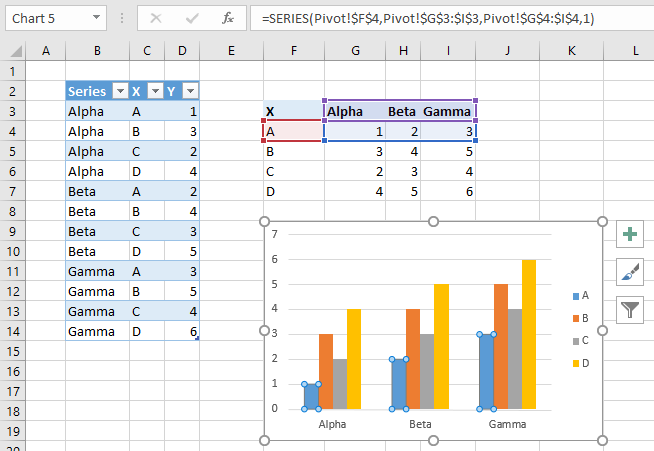
Working with Pivot Charts in Excel - Peltier Tech Blog
Excel Pivot Table Subtotals - Contextures Excel Tips 01/02/2022 · Creating Pivot Table Subtotals . If your pivot table has only one field in the Row Labels area, you won't see any Row subtotals. In the pivot table shown below, Service is in the Row Labels area, Lead Tech is in the Column Labels area, and …

Pivot Table Tip- Assign The Correct Row And Column Labels Quickly - How To Excel At Excel
multiple fields as row labels on the same level in pivot table Excel ... multiple fields as row labels on the same level in pivot table Excel 2016 I am using Excel 2016. I have data that lists product models along with relevant data and also production volumes by month. Part of the relevant data are about 5 common part columns with the part # that applies to each model under the appropriate column.

How To Create A Pivot Table With Multiple Columns And Rows | Cabinets Matttroy
Excel tutorial: How to rename fields in a pivot table Either right-click on the field and choose Value field settings, or click Field Settings on the Options Tab of the PivotTable Tools ribbon. Here, you can see the original field name. In contrast to value fields, Row and Column label field names will be identical to the name in the field list. In fact, they are linked, as we'll see in a minute.
Repeat Pivot Table Labels in Excel 2010 – Excel Pivot Tables
vba sorting pivot table columns by column field label (a date) Hi all, I have a pivot table with multiple row fields and multiple column fields. One of the column fields is a Date and I need some VBA that will auto-sort the columns into ascending order by the Date column field. E.g., if the first four column labels are "2-Jun-2010, 13-May-2009...

How to Make a Pivot Table in Excel | Itechguides.com
Change Blank Labels in a Pivot Table - Contextures Blog You can type any text to replace the (Blank) entry, even a space character, but you can't clear the cell and leave it empty: Select one of the Row or Column Labels that contains the text (blank). Type N/A in the cell, and then press the Enter key. Note: All other (Blank) items in that field will change to display the same text, N/A in this ...
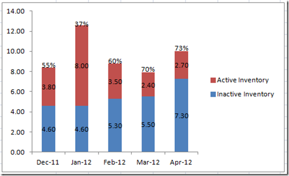
Excel Dashboard Templates How-to Put Percentage Labels on Top of a Stacked Column Chart - Excel ...
How to add column labels in pivot table [SOLVED] Feb 23, 2015 · Re: How to add column labels in pivot table Here are the steps 1. Add a helper column showing Month Text Just as I have done in Column H 2. Now insert a Pivot Table 3. Put Fields in there required sections in the Pivot table Field List Window just as I have done . 4.

pivot table - Excel PivotTable Remove Column Labels - Super User
Format column labels in pivot table | MrExcel Message Board Move the field to row labels. Point to the top edge of the field button until the pointer changes to , and then click. Format it and move it back to column labels You must log in or register to reply here. Similar threads VBA to Filter Column Labels of a Pivot Table SanjayGulatiMusafir Nov 25, 2021 Excel Questions Replies 0 Views 204 Nov 25, 2021
MS Excel 2011 for Mac: Display the fields in the Values Section in multiple columns in a pivot table
Pivot table row labels in separate columns • AuditExcel.co.za Our preference is rather that the pivot tables are shown in tabular form (all columns separated and next to each other). You can do this by changing the report format. So when you click in the Pivot Table and click on the DESIGN tab one of the options is the Report Layout. Click on this and change it to Tabular form.
Show Text in a Pivot Table Values Area - Excel Pivot TablesExcel Pivot Tables
Hide Excel Pivot Table Buttons and Labels Right-click any cell in the pivot table In the pop-up menu, click PivotTable Options In the PivotTable Options dialog box, click the Display tab To hide all of the expand/collapse buttons in the pivot table: Remove the check mark from the option, Show expand/collapse buttons
Post a Comment for "45 excel pivot table column labels"